Writing Queries with Kusto Query Language (KQL)

Kusto Query Language (KQL) is a powerful tool to explore data, designed to query structured, semi-structured, and unstructured data. It has a user-friendly syntax and supports filterings, aggregations, joins, and creating visualizations like charts and graphs, making it ideal for querying logs, metrics and telemetry. In this article, I present how to write queries using KQL.
KQL allows users to retrieve insights from various data sources, and it is a read-only language, so it can not be used to modify or delete data. It is used for monitoring, troubleshooting, and performing analytics, and is supported in a series of Microsoft Products, such as Azure Data Explorer, Microsoft Fabric, Azure Monitor, Microsoft Sentinel, Azure Resource Graph, Microsoft Defender XDR and Configuration Manager (if you want to know what each of these tools are, please check the official Microsoft documentation here).
Playground Environment — Azure Data Explorer (ADX)
Microsoft provides a free playground in Azure Data Explorer that can be used to learn how to work with KQL, for that you only need to have an Azure subscription.
For the next examples in this article, I will be using Azure Data Explorer to demonstrate various queries. However, as mentioned before, many other tools also support KQL.
To create your test environment, do the following:
- Sign in to the Azure Data Explorer web UI
- Then click on “Query” > “Add” > “Connection”:
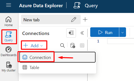
- Then type
helpin the “Connection URI” and click on “Add”:

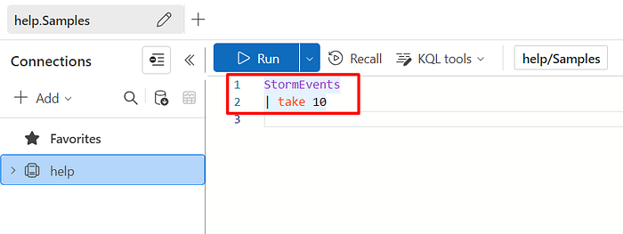
- Then click on the
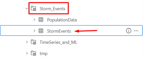
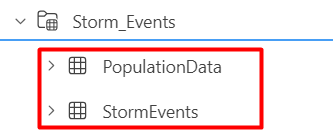
Samplesdatabase, and we can then write some queries to query data from theStormEventstable from theStorm_Eventstable folder:

Query flow
A query begins by specifying the data source, which serves as the foundation by defining the dataset to be analyzed. From this starting point, various operators and commands can be applied in sequence, to filter, transform, and summarize the data, this is indicated visually by the use of a pipe character (|), and you can also combine multiple operations in the same query. Below is a visual representation from Microsoft illustrating this process:

The tabular input is the beginning of the data funnel. This data is piped into the next line, and filtered or manipulated using an operator. The surviving data is piped into the subsequent line, and so on until arriving at the final query output. This query output is returned in a tabular format. (Microsoft Learn)
Writing and Running Queries
You can write your query in the query editor and execute it by clicking on the Run button on the top bar, or pressing Shift + F5 (note that if you have multiple queries written in the editor, only the currently selected one will be executed).
[TIP] Formatting Query
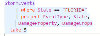
When writing queries in the editor, you can make use of a feature that allows you to format the query. For example, consider the query below:
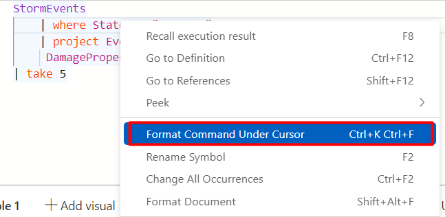
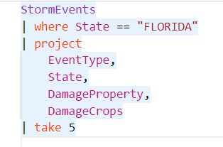
If you right-click and click on “Format Command Under Cursor”, or click Ctrl+K + Ctrl+F, it will automatically format the query for you:
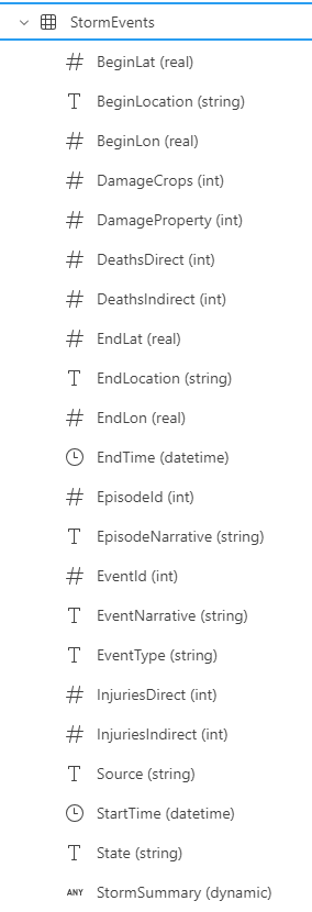
The StormEvents table
The StormEvents is the table we are going to use for most of the examples in this article (later when talking about multi queries, we are going to use the PopulationData table as well).
You can expand the table in the UI and see the columns:
You can also use the getschema together with the table name, to see the table schema:
StormEvents
| getschema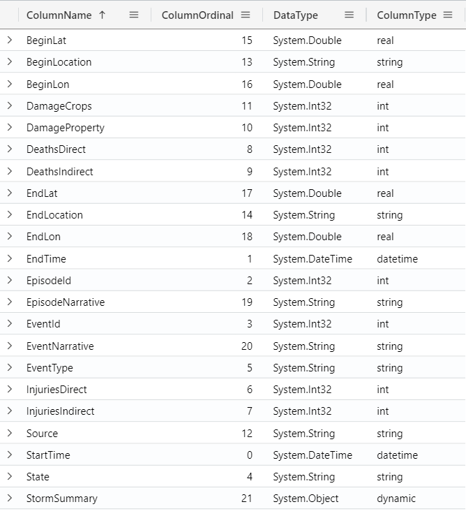
You can click on the column names to sort by the column value:
With the count operator, you can see the number of rows in the table:
StormEvents
| count
You can also combine the getschema and the count to retrieve the number of columns in this table:
StormEvents
| getschema
| count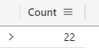
Retrieving all Data
To retrieve all rows and columns from the table, you can simply enter the table’s name and execute it:
StormEvents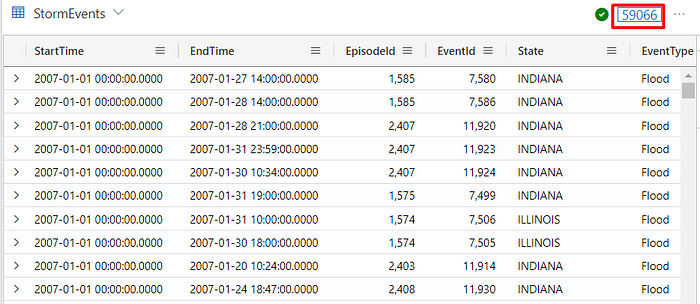
Note that retrieving all rows and columns from a large table without using filters, might take longer and consume more resources, so it is recommended to include some filters or limitations to your queries.
Limiting results — The take operator
To return a specific number of rows, you can use the take operator (or the limit operator). Note that when using the take operator, the records returned are not guaranteed to be consistent unless the source data is sorted. If the dataset is sorted, the take operator will return the first N rows based on the sorting criteria of the data source. Here is an example using the take operator to fetch 5 records:
StormEvents
| take 5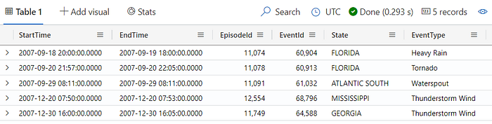
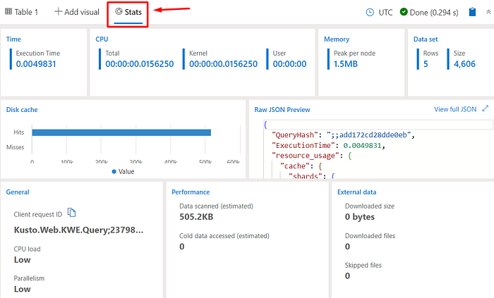
Query Status
In the Stats tab, you can see details of the query you just executed, such as the execution time, the CPU and memory usage, etc. In summary, this is a great way to to check how expensive this query is:
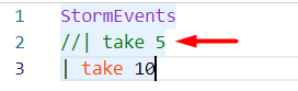
Adding Comments
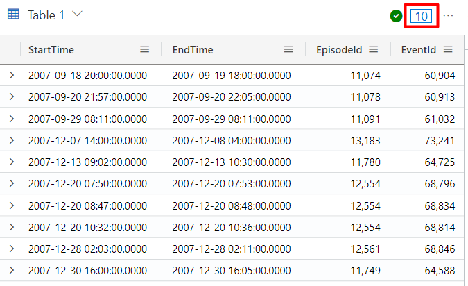
To comment your query or part of it, you can use the //. For example, the query below will return 10 records:
The top operator
The top operator allows you to retrieve a specified number of rows with the highest or lowest values in a specific column. For example, the query below returns the top 10 rows where the DamageProperty has the highest values:
StormEvents
| top 10 by DamageProperty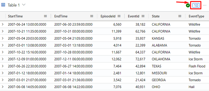
The ascending and descending operators
You can also specify if you want the results to be returned in ascending (asc) or descending (desc) order. By default, the data is always returned in descending order, so using the desc operator is not really required, but it can give more clarity to your query.
For example, the query below returns in ascending order (asc), the top 10 rows which DamagePropery is bigger than 0 (I will explain about the where operator next):
StormEvents
| where DamageProperty > 0
| top 10 by DamageProperty asc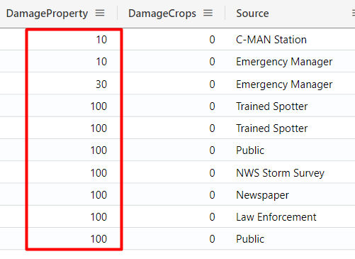
The query below returns the top 10 rows in descending order (desc):
StormEvents
| top 10 by DamageProperty desc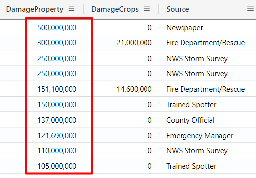
Filtering results — The where operator
To filter records, the where operator can be used. Let’s say you want to filter the records to only show data from Florida. For that, we can use the where operator to filter by the desired State:
StormEvents
| where State == "FLORIDA"
Similar to SQL, you can also combine more filters, for example, to retrieve records from Florida and DamageProperty is bigger than 1500000. You can do that using the and or using another where:
StormEvents
| where State == "FLORIDA"
    and DamageProperty > 1500000

// or

StormEvents
| where State == "FLORIDA"
| where DamageProperty > 1500000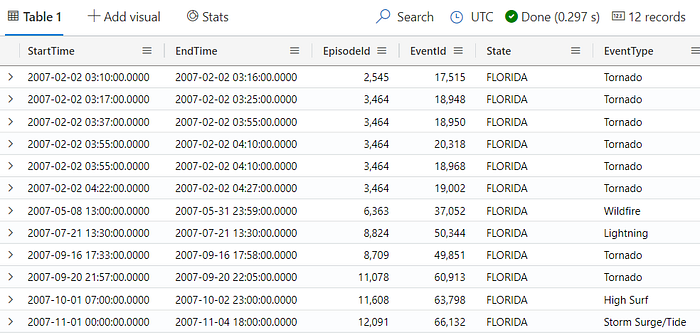
You can also filter using the in operator, in order to filter by multiple values, for example:
StormEvents
| where State in ("FLORIDA", "TEXAS", "OHIO")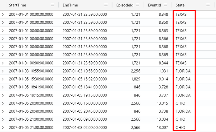
The negation operator
You can also filter using the negation operator !, to negate a condition or to check the absence of a value. For example, if you want to exclude records from Florida:
StormEvents
| where State != "FLORIDA"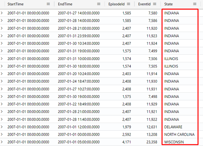
The negation operator can be used in combination with multiple other operators. For example, you can use it with the in operator (and many other operators) to filter out records where the state is Florida or Indiana:
StormEvents
| where State !in ("FLORIDA", "INDIANA")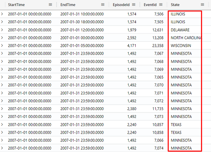
Returning only specific columns — The project operator
The project operator is used to display only the columns you want to be returned. This can be useful to reduce the amount columns displayed, which can be handy when you have multiple columns that are not relevant to your investigation.
For example, the query below will return only the columns added to the project statement:
StormEvents
| where State == "FLORIDA"
| project
    EventType,
    State,
    DamageProperty,
    DamageCrops
| take 5
Renaming columns with project-rename
To rename a column, the project-rename operator can be used. For example, in the query below we are renaming EventType to Event:
StormEvents
| project-rename Event = EventType
| project State, Event
| take 10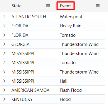
Reordering columns with project-reorder
The project-reorder operator allows you to rearrange the columns in the result. For example, the query below will return the State and EventType as the first columns:
StormEvents
| project-reorder State, EventType
| take 10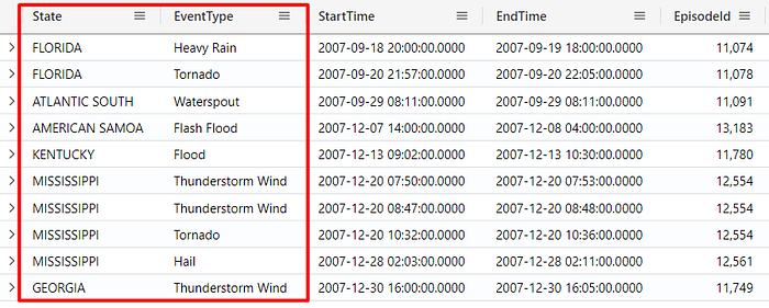
The project away operator
The project awayoperator can be used to specify which columns to exclude from the output table, for example, consider the results below:
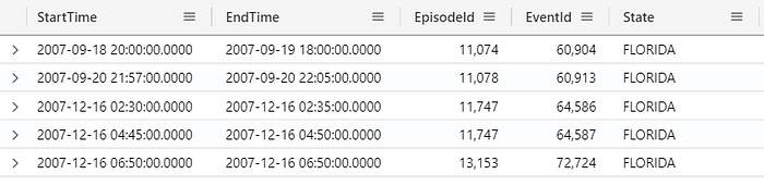
If you do not want to see StartTime and EndTime anymore, you can add these columns to the project-away, and they will not be displayed:
StormEvents
| where State == "FLORIDA"
| project-away
    StartTime,
    EndTime
| take 5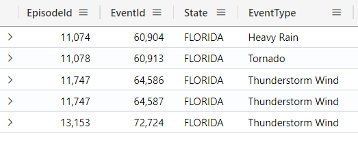
Note that StartTime and EndTime are not present anymore on the result.
Returning new columns with the extend operator
The extend operator can be used to create calculated columns and append them to the result set. For example, you can sum two values and set it to a new column which will be added at the end of the results:
StormEvents
| where State == "FLORIDA"
| extend TotalDamage = DamageProperty + DamageCrops
| take 5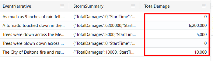
The difference between extend and project, lies in how they handle columns in the results. The extend adds a new column (in the previous example, Damage), and when using project it will only return the specified column.
[Tip] You can also make use of the extend operator to create a specific column/value that can be used as a filter in another query (we will see how to work with multiple queries later):
StormEvents
| project
    State,
    EventType,
    PropertyDamage = DamageProperty,
    Test = true
| take 10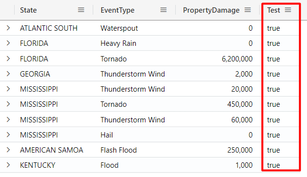
The case function
The case function is used to evaluate multiple conditions and return specific results based on those conditions. It can be used to create calculated columns or perform conditional transformations in queries. For example, the query below categorizes the season in which each storm event happened:
StormEvents
| extend Season = case(
    monthofyear(StartTime) in (12, 1, 2), "Winter",
    monthofyear(StartTime) in (3, 4, 5), "Spring",
    monthofyear(StartTime) in (6, 7, 8), "Summer",
    monthofyear(StartTime) in (9, 10, 11), "Autumn",
    "Unknown"
)
| project StartTime, EventType, Season
Dynamic columns
Note that the column StormSummary from the StormEvents table, has a dynamic type:
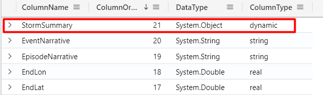
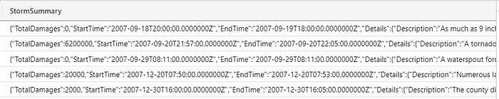
We have JSON value on this column:
With that said, we can also access the properties within this JSON, and ADX also provides intelliSense for it:
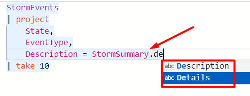
For example, the query below returns the Description property from the JSON:
StormEvents
| project
    State,
    EventType,
    Description = StormSummary.Details.Description
| take 10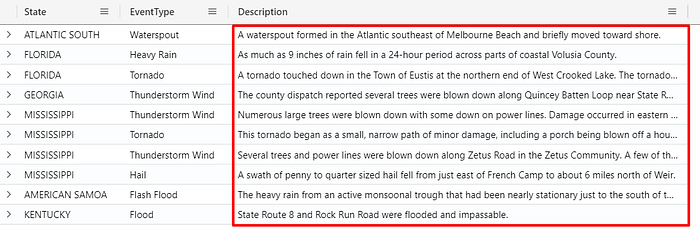
The evaluate operator
The evaluate operator is a feature that applies advanced functions or algorithms to the data. It allows you to use specific plug-in features or statistical methods that are not built into the standard operators of KQL. In the next topic, I’m going to present how to use the evalute operator, using the bag_unpack function.
The bag_unpack function
The bag_unpack function is used to unpack a column of type dynamic (like a JSON stored in a column), by treating each property as a column. For example, consider the StormSummary column:
StormEvents
| take 10
| project StormSummary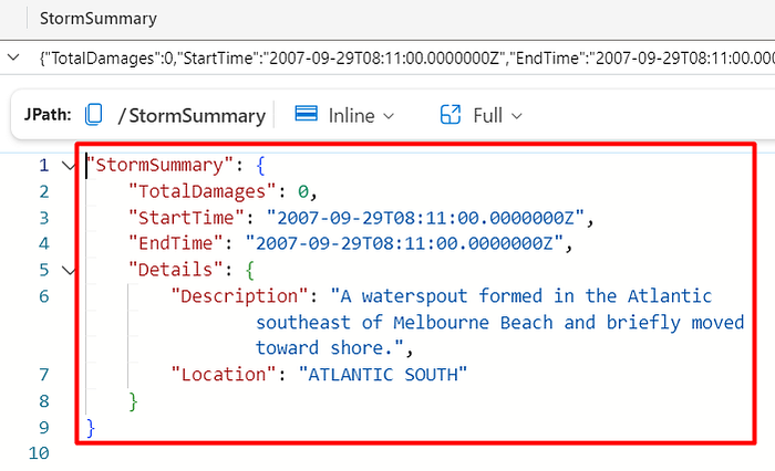
We can use the bag_unpack function to retrieve each of these properties as a column:
StormEvents
| project StormSummary
| take 10
| evaluate bag_unpack(StormSummary)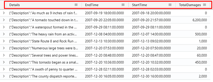
Note that this operator comes right after the evaluate operator. The evaluate operator is a tabular operator that allows you to invoke query language extensions known as plugins. To check other plugins available, check this Microsoft Documentation page.
The sort by operator
The sort byoperator (or order by operator) allows you to order your data based on one or more columns, either in ascending (asc) or descending (desc) order. In the example below, the query retrieves storm events in Florida and sorts the results by EventType alphabetically (ascending) and, within each event type, by DamageProperty in descending order (highest to lowest):
StormEvents
| where State == "FLORIDA"
| project
    EventType,
    State,
    DamageProperty,
    DamageCrops
| sort by
    EventType asc,
    DamageProperty desc
| take 10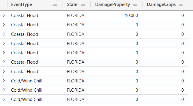
Note that adding the desc in this case is not mandatory, as by default it will be sorted in descending order.
The has operator
The has operator is a case-insensitive search that matches a full term. For example, if you search for “wind”, it will bring rows that have the word “wind”:
StormEvents
| where EventType has "wind"
| project StartTime, EventType, DamageProperty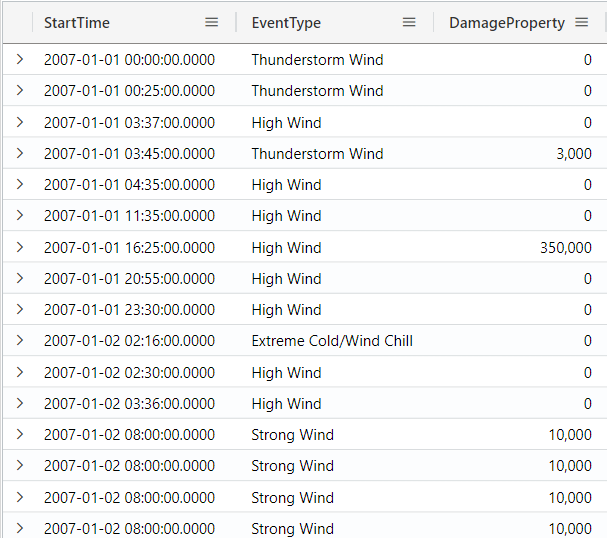
If you want to filter considering case sensitive, you can use has_cs for example:
StormEvents
| where EventType has_cs "Wind"
| project StartTime, EventType, DamageProperty
The contains operator
The contains operator is similar to has, but it matches on any substring. For example, if you search for “free”, it will bring “Freezing fog” and “Fros/Free”:
StormEvents
| where EventType contains "free"
| project StartTime, EventType, DamageProperty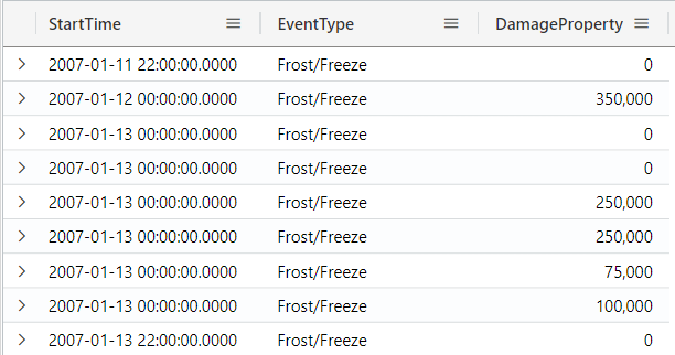
Similar to the hasoperator, you can also filter considering case sensitive, using contains_cs:
StormEvents
| where EventType contains_cs "Free"
| project StartTime, EventType, DamageProperty
The
hasoperator is more performant than thecontainsoperator, so you should usehaswherever you have a choice between the two. (Microsoft Docs)
Filtering by date and time — The between operator
If you need to filter records by a specific time range, you can use the between operator, and specify the start and end date you want to filter, using the syntax <column-name> between (<lower-bound> .. <upper-bound>), for example:
StormEvents
| where StartTime between (datetime(2007-01-01) .. datetime(2007-02-01))
    and State == "FLORIDA"
| project StartTime, EventType, DamageProperty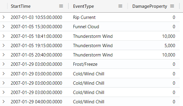
Mathematical Operations with DateTime fields
When working with DateTime columns, you can perform mathematical operations with these columns. For example, the query below calculates the duration of each event (EndTime - StartTime):
StormEvents
| take 10
| extend Duration = EndTime - StartTime
| project EventType, Duration, StartTime, EndTime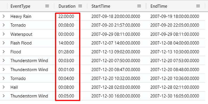
The distinct operator
The distinct operator can be used to list the distinct values of a specific column. For example, the query below lists all the Event Types in the state of Florida:
StormEvents
| where State == "FLORIDA"
| distinct EventType
| sort by EventType asc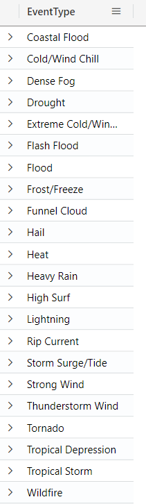
Aggregating Data — The summarize operator
The summarize operator is used to aggregate data. It groups data based on one or more columns and applies aggregation functions like count, sum, avg, min, max, and others. For example, the query below counts the number of events per state:
StormEvents
| summarize EventCount = count() by State
| sort by EventCount
The dcount() and countif() functions
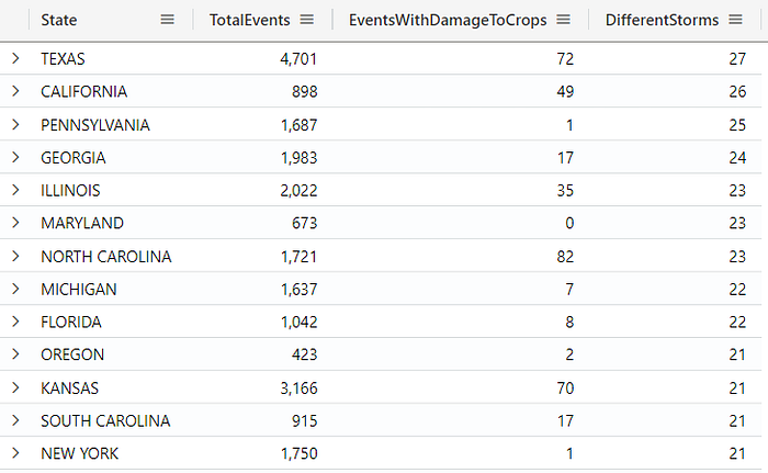
The dcount() and countif() functions is used to perform more advanced count operations. The countif() function counts records for which a predicate is true. The dcount() function, allows you to count distinct types of events. For example, check the query below:
StormEvents
| summarize TotalEvents = count(),
    EventsWithDamageToCrops = countif(DamageCrops > 0),
    DifferentStorms = dcount(EventType) by State
| sort by DifferentStorms
This query returns the number of events, the number of events that caused damage and the number of storms (event types) that happened in each state.
Note that if you do not specify a column name for the columns, a default name will be automatically added, for example, consider the query below where no name is being specified for the columns in the summarize operator:
StormEvents
| summarize count(),
    countif(DamageCrops > 0),
    dcount(EventType) by State
| sort by count_
The render operator
The render operator in KQL is used to define how the output of a query is visualized when displayed. It allows you to customize the visual representation of your data, such as tables, charts, or time series. This operator goes at the end of the query, and can only be used with queries that produce a single tabular data stream result.
Within the render operator, you can specify which type of visualization to use, such as columnchart, barchart, piechart, and others (you can see more options on this Microsoft Documentation page). You can also optionally define different properties of the visualization, such as the x-axis or y-axis. The query below will display a pie chart with the percentage of events per state:
StormEvents
| summarize
    TotalEvents = count(),
    DifferentStorms = dcount(EventType)
    by State
| render piechart
You can also add a title to the char by specifying the title in the query:
| render piechart with(title="Events per state")In Data Explorer UI, you can also switch the chart type (or you can also use the barchar with the render):
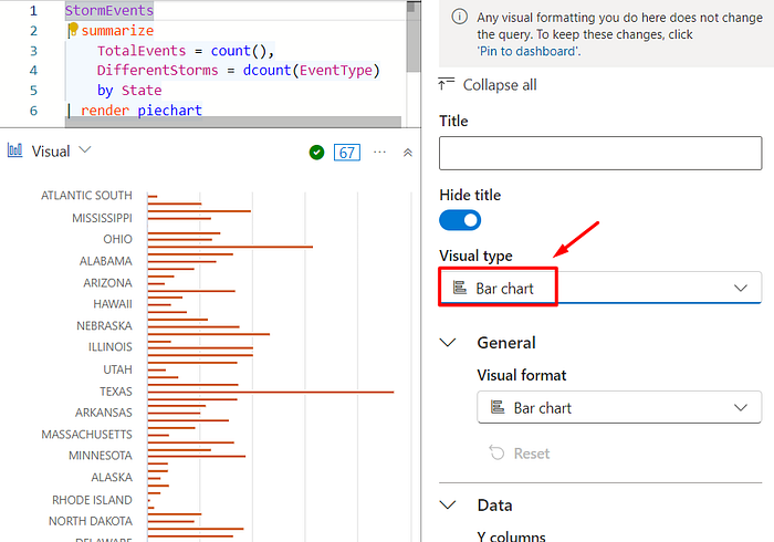
Note that you can hover the mouse over the chart to see more details, and you can also toggle the values to display only that specific data in the chart, for example:
StormEvents
| summarize TotalEvents = count(),
    EventsWithDamageToCrops = countif(DamageCrops > 0),
    DifferentStorms = dcount(EventType) by State
| sort by DifferentStorms
| take 5
| render barchart
Grouping Data — The bin operator
The bin operator is used to group values into fixed-size “bins” or intervals. This can be useful for aggregating data over time or numeric ranges. The bin value can be a number, date, or timespan, and the structure is bin(value, roundTo). For example, the following query bins StormEvents data by the interval of one hour, to count the number of events in each bucket:
StormEvents
| summarize EventCount = count() by bin(StartTime, 1h)
| sort by StartTime asc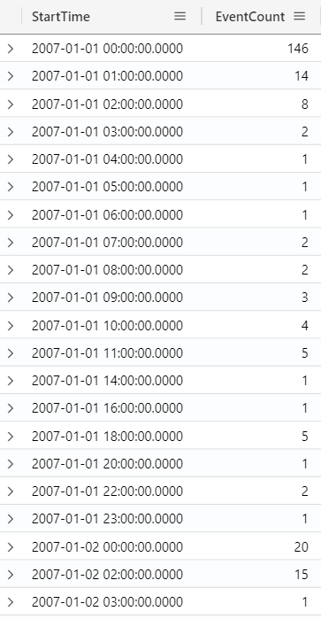
You can also use it to filter by each day, for example:
StormEvents
| summarize EventCount = count() by bin(StartTime, 1d)
| sort by StartTime asc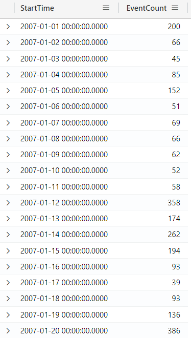
The sum operator
The sum operator is an aggregation function that can be used to sum values. For example, in the query below I’m calculating the total damage for Florida, by summing the DamageProperty with DamageCrops:
StormEvents
| where State == "FLORIDA"
| extend TotalDamage = DamageProperty + DamageCrops
| summarize sum(TotalDamage) by State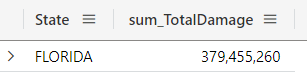
You can also use the sumif(), which allows you to specify a predicate (a condition) as a parameter, and the sum will be done based on what you specify, for example, in the query below it is specified that it will only sum values bigger than 0 (this is only for demonstration purposes):
StormEvents
| where State == "FLORIDA"
| extend TotalDamage = DamageProperty + DamageCrops
| summarize sumif(TotalDamage, TotalDamage > 0) by State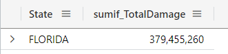
The average Function
The avg() function sums up all the numeric values in the specified column and divides the total by the number of rows (excluding null values).
If the column contains null or empty values, they are ignored in the calculation. For example, the query below returns the average damage in Florida:
StormEvents
| extend TotalDamage = DamageProperty + DamageCrops
| where TotalDamage > 0
    and State == "FLORIDA"
| summarize avg(TotalDamage) by EventType
| sort by avg_TotalDamage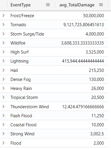
Note that the column avg_TotalDamage was automatically created for us (the column name is based on what we see the line which contains the avg function).
Similar to the previous example, you can also use the avgif() function, which is similar to the avg() function, but it will only calculate results for which the predicate (condition) is true.
The min and max operators
The min() and max() aggregation functions can be used to return minimum and maximum values. You can specify to the function, the column you want to retrieve the min/max value. For example, we can run the following query to return the minimum and maximum damage for Florida:
StormEvents
| extend TotalDamage = DamageProperty + DamageCrops
| where State == "FLORIDA"
    and TotalDamage > 0
| summarize
    MinDamage = min(TotalDamage),
    MaxDamage = max(TotalDamage),
    AverageDamage = avg(TotalDamage)
    by EventType
| sort by MaxDamage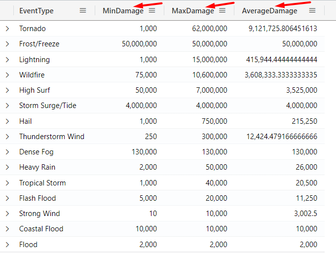
Similar to previous examples, you can also use minif() and maxif().
Using variables with let
The let statement allows you to define variables to organize complex queries. This can be useful to break up complex expressions into multiple parts. It’s possible to use multiple let statements, and each statement must be followed by a semicolon (;).
For example, in the query below I’m specifying a variable for the event location, and using this variable in the query:
let EventLocation = "FLORIDA";

StormEvents
| where State ==  EventLocation
| extend TotalDamage = DamageProperty + DamageCrops
| where TotalDamage > 0
| sort by TotalDamage
| summarize sum(TotalDamage) by EventType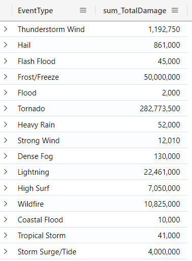
Attention: Note that even though in the query example there is a space between the first line and the third line, when you execute the query, you need to select everything, or remove the empty line.
Adding a query to a variable
You can also assign the result of your query to a variable and then use that variable to perform further queries (Just remember to end the query with a semicolon (;):
let FilteredFloridaDamage = StormEvents
    | where State == "FLORIDA"
    | extend TotalDamage = DamageProperty + DamageCrops
    | where TotalDamage > 0
    | sort by TotalDamage
    | summarize sum(TotalDamage) by EventType;

FilteredFloridaDamage
| where sum_TotalDamage > 50000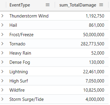
Converting the result to a scalar value
You can also use the toscalar() function, which allows you to extract a single scalar value from a query result. This value can then be used elsewhere in the query as a constant. This can be useful when you want to calculate a value once and reuse it without recalculating it multiple times. For example, consider the query below, which returns the most frequent event type:
StormEvents
| summarize count() by EventType
| top 1 by count_
| project EventType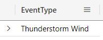
Now you can add this query to a variable and use it in another query. In the query below we are searching for the most frequent event type that happened each month:
let MostFrequentEventType = toscalar(
    StormEvents
    | summarize count() by EventType
    | top 1 by count_
    | project EventType);

StormEvents
| where EventType == MostFrequentEventType
| summarize
    count()
    by
    Date = startofmonth(StartTime)
| sort by Date asc
The format_datetime function
In order to improve the readability of Datetime columns, you can use the format_datetime function to format the date in the way you need. For example, consider the previous query, where we only care about month and year, we can use this function to format this column for us, returning only the necessary information related to the Datetime column:
let MostFrequentEventType = toscalar(
    StormEvents
    | summarize count() by EventType
    | top 1 by count_
    | project EventType);

StormEvents
| where EventType == MostFrequentEventType
| summarize
    EventCount = count()
    by
    Date = format_datetime(startofmonth(StartTime), "MM-yyyy")
| sort by Date asc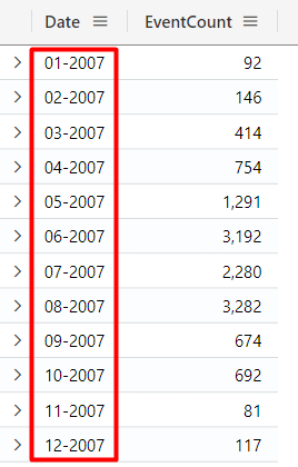
In this Microsoft Documentation page, you can see all possible options that can be used with this function.
Creating a user-defined function
You can define a user-defined function using the let statement, which allows you to create reusable logic that you can use in your queries. For example, in the query below, we created a function named CalculatePercentage, which is used in the query:
let CalculatePercentage = (portion: real, total: real) {
    round(100 * portion / total, 2)
};

StormEvents
| extend TotalDamage = DamageCrops + DamageProperty
| summarize
    TotalEvents = count(),
    TotalDamagingEvents = countif(TotalDamage > 0)
    by EventType
| project
    EventType,
    TotalDamagingEvents,
    TotalEvents,
    Percentage = CalculatePercentage(TotalDamagingEvents, TotalEvents)
| sort by EventType asc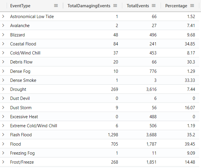
Multi queries with KQL
For this section, we are going to continue using the StormEvents table, and we are also going to use another table, the PopulationData table:
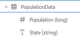
The PopulationData table contains these two columns:
Combining data from multiple tables
KQL allows you to combine data from multiple tables. You can do that by using different operators, such as:
- The
unionoperator: which combines results of two or more tables/queries, into a single output, and it can combine tables even if they have different columns. - The
joinoperator: which supports many different kinds of joins, such asinner,leftouter,rightouter,leftanti,rightanti, etc. - The
lookupoperator: which is a special implementation of ajoin, which optimizes the performance of queries.
The union operator
The union operator is used to combine results of two or more tables/queries, into a single output, and it can combine tables even if they have different columns. This can be useful when you are working with multiple datasets that share common or complementary information. For example, consider the query below, on which we have different filters for each State, and we group them to get the result:
let FloridaEvents = StormEvents
| where State == "FLORIDA"
| extend TotalDamage = DamageProperty + DamageCrops
| where TotalDamage > 1500
| project EventType, State, TotalDamage;

let TexasEvents = StormEvents
| where State == "TEXAS"
| extend TotalDamage = DamageProperty + DamageCrops
| where TotalDamage > 2000
| project EventType, State, TotalDamage;

FloridaEvents
| union TexasEvents
| sort by TotalDamage asc
| take 20
The join operator
The join operator is used to combine data from two tables based on a common key. The output can include data from both tables for matching rows. This is the structure to write joins in KQL:
| join kind = <inform-join> <inform-table> on <inform-key>Note that if you want to reduce the number of rows being considered by the join, you should apply the take operator before the join, and if you want to ensure the join processes all matching rows and then randomly sample the results, you should apply take operator after the join.
For our example, we can use the State column to join the StormEvents and the PopulationData tables.
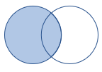
The leftouter join
The leftouter join returns all rows from the left table, and only matching rows from the right table, and if there are no records on the right table, it will still return the record on the left, and you will see empty value for columns on the right table:
For example, consider the query below:
StormEvents
| take 10
| join kind = leftouter (PopulationData) on State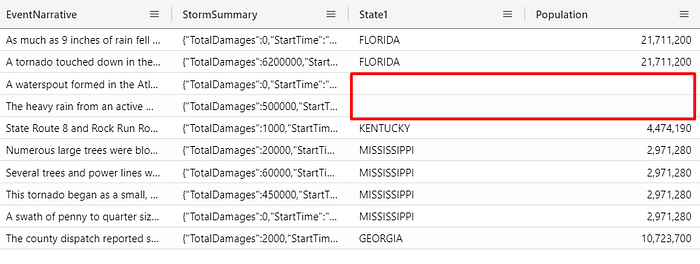
You can see on the result that we have some rows without value on these columns, and the reason is because there is no record for the State we specified the join, in the PopulationData table (right table).
Similar to the leftouter, you can also make use of the rightouter, which returns all records from the right table and only matching rows from the left table.
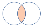
The inner unique join
By default, when not specifying the kind of join, the innerunique join is applied. This kind of join returns all deduplicated rows from the left table that match rows from the right table:
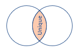
For example, consider the query below:
StormEvents
| take 10
| join kind = innerunique (PopulationData) on State
| project State, State1

// or

StormEvents
| take 10
| join (PopulationData) on State
| project State, State1
The innerunique operator only returns rows that have a record in both tables, but then it does a deduplication on the left side table:
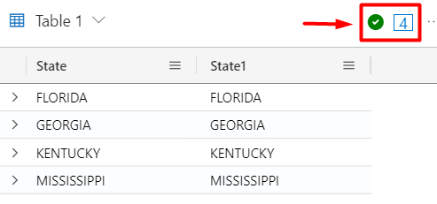
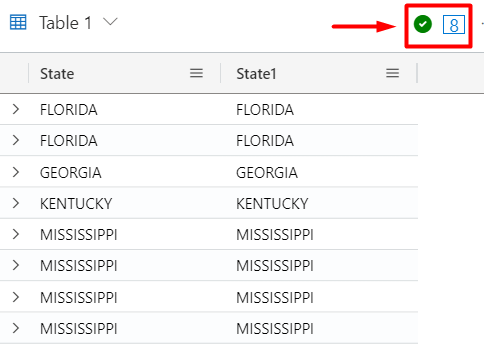
The inner join
The inner operator is used to retrieve rows from two tables where there is a match based on the join condition. With the inner join, only matching rows from both tables will be returned:
For example, consider the query below:
StormEvents
| take 10
| join kind = inner (PopulationData) on State
| project State, State1
This results in 8 rows, because it returns all combinations that match:
The difference between inner vs innerunique
With the inner join, it ensures that all rows from both tables (left and right) are included in the result if they satisfy the join condition. If multiple rows in one table match a single row in the other table, all combinations of matches will appear in the result.
With the innerunique join, it ensures that each row from the left table matches with at most one row from the right table. For each row in the left table, only one matching row from the right table is included. If there are multiple matches, an arbitrary one is chosen.
The leftanti join
The leftanti join, returns all rows from the left table that do not match records from the right table:

For example, the query below returns the State value that exists in the left table (StormEvents) and does not exist in the right table (PopulationData):
StormEvents
| take 10
| join kind = leftanti (PopulationData) on State
| project State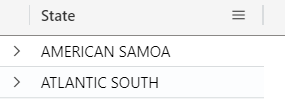
Similar to the leftanti, you can also make use of the rightanti, which returns all records from the right table and only matching rows from the left table (which will result in all the States, except these two from previous example, that are not present in the right table).
The fullouter join
The fullouter join returns all records from both tables, with unmatched cells populated with null. This kind of join ensures that you retain every record from both sides.

For example, consider the query below, which ensures you get a complete set of data, where you can see both matched and unmatched records from both sides:
StormEvents
| take 10
| join kind = fullouter (PopulationData) on State
| project State, State1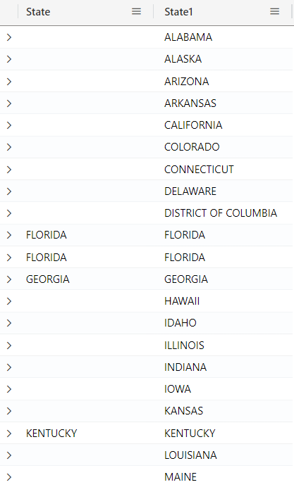
If you want to know more about the other kinds of joins, check this Microsoft documentation page.
The materialize function
The materialize function caches the result of a subquery when it runs, so other queries or parts of the query can reference the cached result, making it easier and faster to reference in subsequent operations. This can be useful for optimizing your queries and improving readability.
For example, consider the query below, on which we cache (materialize) the results of the join with StormEvents and PopulationData tables, and we use this cached result in a subsequent query, on which we summarize some columns and apply a filter. This query allows you to identify and analyze the states most affected by storms, returning both the total of the damage and the population size:
let CachedStormPopulationData = materialize(
    StormEvents
    | join kind=inner (PopulationData) on State
    | project State, EventType, DamageProperty, DamageCrops, Population
);

CachedStormPopulationData
| summarize
    EventCount = count(),
    TotalDamage = sum(DamageProperty) + sum(DamageCrops),
    TotalPopulation = sum(Population)
    by
    State
| where TotalDamage >= 500000
| order by TotalDamage desc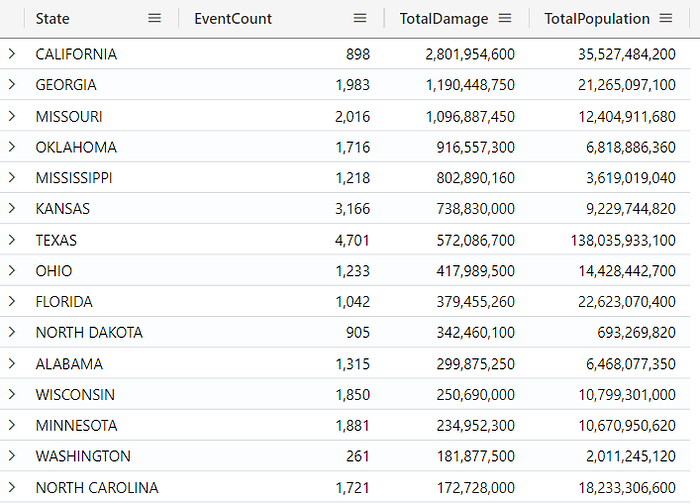
Conclusion
As presented, Kusto Query Language (KQL) is a powerful language used to query data from multiple data sources, and it is used by a range of products like Azure Data Explorer, Azure Monitor, and others. It is commonly used for querying telemetry, metrics and logs, uses a user-friendly syntax and supports many types of filtering, aggregations, joins, and visualizations. Whether you are monitoring infrastructure, performing analysis, or simply working with data, KQL allows you to efficiently extract insights.
In this article, we created the playground environment, which is a great place to play with KQL, and we started with how to write and execute simple queries and delved into multiple operators, illustrated using practical examples, demonstrating how KQL can filter, transform, and summarize data to generate meaningful insights.
Thanks for reading!